A step-by-step instruction on how to make a chart in Excel

In our life, we can not do without various comparisons. Figures - it's not always convenient for perception, that's why a man invented diagrams.

The most convenient program for creating graphs of different kinds is Microsoft Office Excel. How to create a diagram in Excel, and will be discussed in this article.

This process is not so complicated, it is only necessary to follow a certain algorithm.

Step-by-step instructions on how to make a chart in Excel

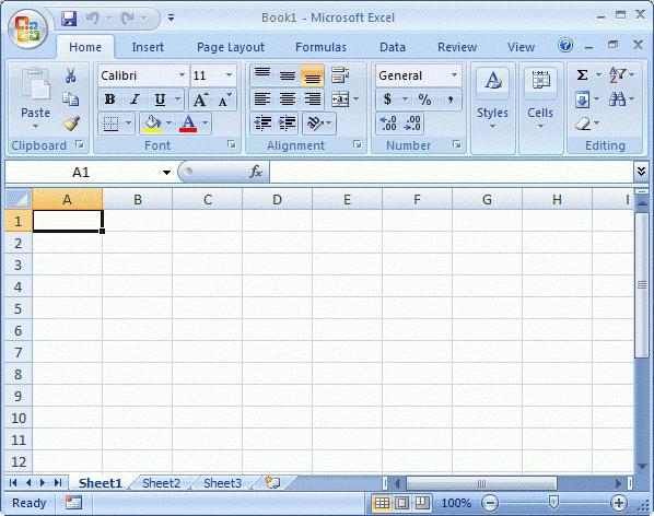
1. Open the document: the Start button - All program list - the folder "Microsoft Office" - the document "Excel".

2. Create a table of the data you want to visualize on the diagram. Select the range of cells containing numeric data.

3. Call the "Wizard for the construction of graphs and diagrams." Commands: "Insert" - "Diagram".

The dialog box for the wizard will appear on the screen. It will help you to decide how to make a diagram in Excel. But for this work it is necessary to perform four simple steps.

1. The first step is to choose the type of chart. As can be seen from the opened list, there is a wide variety of these types: graph with areas, bubble diagram, histogram, surface and so on. Non-standard chart types are also available for selection. An example of a graphical display of the future graph can be seen in the right half of the window.

2. The second step in order to answer the question,how to make a chart in Excel, is the input of the data source. We are talking about the very plate, which was mentioned in the second paragraph of the first part of the article. On the "Row" tab, you can specify the name of each row (column of the table) of the future chart.

3. The most voluminous item number 3: "Chart parameters." Let's go through the tabs:

• Headings. Here you can assign the labels of each axis of the chart and give a name to it.

• The axes. Allows you to select the type of axes: time axis, category axis, automatic type detection.

• Lines of the grid. Here you can set or, vice versa, remove the main or intermediate lines of the grid graph.

• Legend. Allows you to display or hide a legend, and select its location.

• Data table. Adds a data table to the plotting area of ​​the future chart.

• Data captions. Includes data signatures and provides a choice of a separator between the indicators.

4. The last and shortest step on the way to building a chart in Excel is choosing the placement of the future graph. There are two options to choose from: the source or the new sheet.

5. After all the necessary fields of the dialog windows of the Chart Wizard are filled, we boldly press the "Finish" button.

Your creation appears on the screen. And although the Chart Wizard allows you to view the future schedule at each stage of your work, you eventually need to correct something.

For example, by right-clicking a couple of times in the(but not by itself!), you can make the background on which the chart is located, color or change the font (face, size, color, underlining).

When you double-click the same right buttonmouse on the chart lines you can format the grid lines of the chart itself, set their type, thickness and color and change a lot of other parameters. The construction area is also available for formatting, or rather, for coloring.

We hope that you have received the most understandable and simple answer to your question: "How to make a diagram in Excel?". It's very simple, if you follow the above instructions. We wish you success!

</ p>